1.4. El producto vectorial

En esta sección vamos a aprender a manejar el producto vectorial, una aplicación que, dados dos vectores no nulos en \(\mathbb{R}^3\), nos permite calcular un tercer vector ortogonal a los dos dados.

1.4.1. Producto vectorial. Definición y propiedades

Definition (Producto vectorial)

Sean \(\mathbf{u}=\left( u_{1}, u_{2}, u_{3} \right) = u_{1}\mathbf{i} + u_{2}\mathbf{j} + u_{3}\mathbf{k}\) y \(\mathbf{v}=\left( v_{1}, v_{2}, v_{3} \right) = v_{1}\mathbf{i} + v_{2}\mathbf{j} + v_{3}\mathbf{k}\) dos vectores no nulos. Definimos su producto vectorial como el vector

\[ \mathbf{u} \times \mathbf{v} = \left( u_{2}v_{3}-u_{3}v_{2} \right)\mathbf{i} - \left( u_{1}v_{3}-u_{3}v_{1} \right)\mathbf{j} + \left( u_{1}v_{2}-u_{2}v_{1} \right)\mathbf{k}. \]

Suele representarse, aprovechando la notación de determinantes, y desarrollando por los menores de la primera fila,

\[\begin{split} \mathbf{u} \times \mathbf{v} = \left| \begin{array}{ccc} \mathbf{i} & \mathbf{j} & \mathbf{k} \\ u_{1} & u_{2} & u_{3} \\ v_{1} & v_{2} & v_{3} \end{array} \right| = \left|\begin{array}{cc} u_{2} u_{3} \\ v_{2} v_{3} \end{array}\right| \mathbf{i} - \left|\begin{array}{cc} u_{1} u_{3} \\ v_{1} v_{3} \end{array}\right| \mathbf{j} + \left|\begin{array}{cc} u_{1} u_{2} \\ v_{1} v_{2} \end{array}\right| \mathbf{k}. \end{split}\]

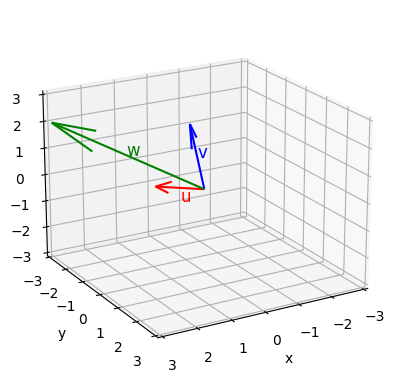
Veamos un ejemplo, aprovechando la función np.cross de Numpy, que calcula directamente el producto vectorial:

import numpy as np
import matplotlib as mp
import matplotlib.pyplot as plt

# Definimos los vectores u y v
u = np.array([2, 1, 1])
v = np.array([1, 1, 3])

# Calculamos su producto vectorial con la función, de Numpy, np.cross
w = np.cross(u,v)

display(w)

# Inicialización de la representación 3D
fig = plt.figure()
ax = fig.add_subplot(111, projection='3d')

# Representación de los vectores
ax.quiver([0], [0], [0], np.array([u[0], v[0], w[0]]), np.array([u[1], v[1], w[1]]), 
          np.array([u[2], v[2], w[2]]), color=['r','b','g','r','r','b','b','g','g'])

# Añadimos etiquetas a los vectores
ax.text(u[0]/2, u[1]/2, u[2]/2-0.5, 'u', fontsize=12, color='r')
ax.text(v[0]/2, v[1]/2, v[2]/2, 'v', fontsize=12, color='b')
ax.text(w[0]/2, w[1]/2, w[2]/2, 'w', fontsize=12, color='g')

# Ajuste de los límites de los ejes
ax.set_xlim([-3,3])
ax.set_ylim([-3,3])
ax.set_zlim([-3,3])

# Etiquetas de los ejes
ax.set_xlabel('x')
ax.set_ylabel('y')
ax.set_zlabel('z')

# Orientamos los ejes
ax.azim = 60
ax.elev = 20

plt.show()

array([ 2, -5,  1])

Veamos a continuación algunas propiedades del producto vectorial:

Property (Propiedades algebraicas del producto vectorial)

Sean \(\mathbf{u}\), \(\mathbf{v}\) y \(\mathbf{w} \in\mathbb{R}^{3}\) y sea \(c\in\mathbb{R}\). Se cumple

1. \(\mathbf{u}\times\mathbf{v} = -\left( \mathbf{v}\times\mathbf{u} \right)\) (anticonmutativa).

2. \(\mathbf{u}\times\left( \mathbf{v} + \mathbf{w} \right) = \left(\mathbf{u}\times\mathbf{v}\right) + \left(\mathbf{u}\times\mathbf{w}\right)\) (distributiva respecto a la suma).

3. \(c \left( \mathbf{u} \times \mathbf{v} \right) = \left(c \mathbf{u}\right) \times \mathbf{v} = \mathbf{u} \times \left(c \mathbf{v}\right)\).

4. \(\mathbf{u} \times \mathbf{0} = \mathbf{0} \times \mathbf{u} = \mathbf{0}\).

5. \(\mathbf{u} \times \mathbf{u} = \mathbf{0}\).

6. \(\mathbf{u}\cdot\left( \mathbf{v} \times \mathbf{w} \right) = \left( \mathbf{u} \times \mathbf{v} \right) \cdot \mathbf{w}\).

Property (Propiedades geométricas del producto vectorial)

Sean \(\mathbf{u}\), \(\mathbf{v} \in\mathbb{R}^{3}\) vectores distintos de \(\mathbf{0}\) y sea \(\theta\) el ángulo entre ellos. Se cumple

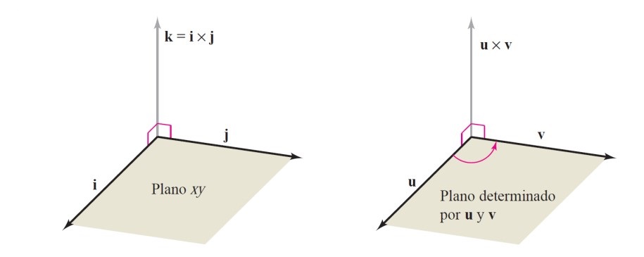
1. \(\mathbf{u}\times\mathbf{v}\) es ortogonal tanto a \(\mathbf{u}\) como a \(\mathbf{v}\).

2. \(\| \mathbf{u}\times\mathbf{v} \| = \| \mathbf{u} \| \| \mathbf{v} \| \sin\theta\).

3. \( \mathbf{u}\times\mathbf{v} = \mathbf{0}\) si y sólo si \(\mathbf{u}\) y \(\mathbf{v}\) son paralelos (es decir, si \(\exists c\in\mathbb{R}\) tal que \(\mathbf{v} = c \mathbf{u}\)).

4. \(\| \mathbf{u}\times\mathbf{v} \|\) es igual al área del paralelogramo que tiene a \(\mathbf{u}\) y a \(\mathbf{v}\) como lados adyacentes.

Para ver la orientación de \(\mathbf{u}\times\mathbf{v}\) se puede utilizar la regla del sacacorchos entre \(\mathbf{u}\) y \(\mathbf{v}\), como se muestra en la siguiente figura: